An investor is offered different assets or securities in a given market, each with a varied rate of return depending on the underlying risk.
How to choose an asset, a set of various assets, or a security investment that best optimizes risk and return on investment while maximizing expected utility is a practical concern for rational investors. But we can get around this problem by using portfolio optimization with the mean-variance method.
In this post, we’ll explore the concept of portfolio optimization and demonstrate how to create some standard portfolios for portfolio optimization using the mean-variance approach.
What is Portfolio Optimization?
Let’s first understand what portfolio optimization is. Portfolio optimization in investing refers to the process of choosing assets in a way that maximizes return while minimizing risk. For example, to ensure they make the highest possible return, an investor might be interested in choosing five stocks from a list of twenty. Private equity investments can be managed and diversified with the help of portfolio optimization techniques. Investing in Bitcoin and Ethereum, among other cryptocurrencies, has recently benefited from the application of portfolio optimization strategies.
The goal of asset optimization in each of these scenarios is to strike a balance between risk and return, with return on a stock being the profits realized over time and risk being the standard deviation in the value of an asset. Numerous portfolio optimization techniques are simply advancements of asset diversification techniques used in investing. The key concept behind this is that diversifying your portfolio o,f assets rather ,than keeping them in the same way reduces your risk.
What is Mean-Variance Optimization?
Investment banks and asset management companies put a lot of effort into finding the best techniques for portfolio optimization. One of the original techniques is known as mean-variance optimization, often known as the Markowitz Method or the HM technique because it was created by Harry Markowitz. It entails assessing an asset’s risk to its expected return and making investments based on that risk/return ratio. Here’s how it functions.
Investors can use a mean-variance analysis as a technique to help disperse risk across their portfolios. In it, the investor calculates the risk of an asset, which is represented by the “variance,” and then compares it with the asset’s expected return. The objective of a mean-variance optimization is to maximize return based on the investment’s risk.
Investors employ mean-variance analysis to make investment decisions. They evaluate how much risk they are ready to accept in exchange for various degrees of profit. They can use mean-variance analysis to determine which investment offers the best return at a particular level of risk or the lowest risk at a particular level of return. They can then investbased of that information. This enables them to diversify their portfolios across various risk levels and choose investments depending on desired returns.
Understanding Mean-Variance Portfolio Optimization
The Mean-Variance Portfolio Theory (MPT)
Mean-Variance Portfolio Theory, often called The Modern Portfolio Theory (MPT), was developed by Harry Markowitz in 1952. Investors can use the key concepts presented in the theory as practical guidelines for building investment portfolios to ensure the highest expected return given a specific amount of risk.
Assumptions of Modern Portfolio Theory
The following are some fundamental presumptions upon which the MPT is based.
- Markets are open and transparent, and investors may obtain all information about the expected return, variances, and covariances of securities or other assets.
- Investors tend to avoid unneeded risks since they are risk-averse. For example, investors like bank deposits over equities since the latter may offer higher returns but come with a high risk of losing money. Bank deposits, however, pay lower returns but are guaranteed.
- Investors are not satisfied, thus they would choose the security with the higher predicted return if presented with two options with the same standard deviation.
- Any amount can be held as an asset.
- A fixed single-time horizon exists.
- There are no transaction fees or taxes.
- Investors based onions exclusively on the basis of variance and expected returns.
- There is a risk-free rate of return in the market, and unlimited cash can be borrowed or invested at this rate.
Now that we have learned our working hypothesis, we may now start to comprehend the intuition behind MPT. To get started, consider a portfolio that has two equities, A and B.
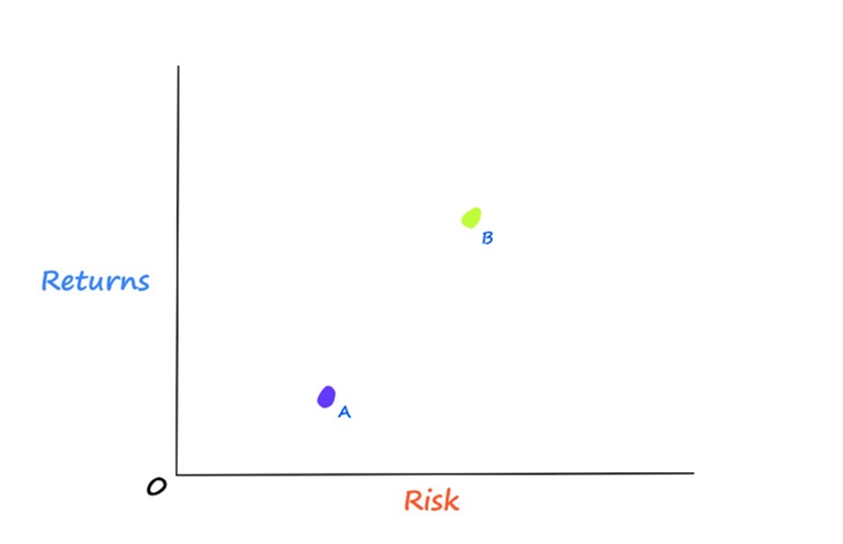
We can observe from the image above that Stock A has lower expected returns and lower risk than Stock B. Before MPT, it was supposed that these two stocks could be combined in any number of linear portfolios.
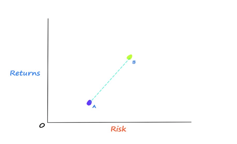
Supposing that there’s a linear relationship among our stocks, all of our potential portfolio combinations should, in theory, fall somewhere along the dotted line in the accompanying image. We would be mistaken, in Markowitz’s opinion. According to Markowitz’s theory, the relationship between our stocks has a curved form known as the efficient frontier rather than being linear. So, our potential portfolio combinations are accurately represented by the efficient frontier.
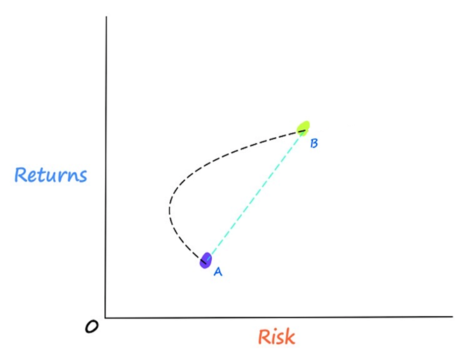
You might now be wondering how this is feasible. All of this efficient frontier is possible by correlation. In order to better understand how correlation gives us the curved shape that represents the portfolio configurations, we must first comprehend how our portfolio returns and portfolio risk are determined.
Portfolio Returns & Risk
In a nutshell, the expected return of the entire portfolio is equal to the proportional sum of the expected returns of the individual assets.
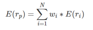
Where:
Wi stands for the ith asset of the portfolio
E(ri) denotes the expected return on i-th asset of the portfolio
This computation of the portfolio’s expected return is based on the same reasoning that leads us to conclude that the relationship between the two stocks is linear. This relationship becomes non-linear when we calculate the risk of our portfolio.
Let us determine the portfolio’s risk, which also represents the variance of the portfolio.
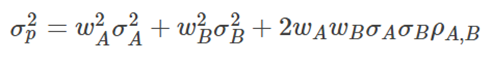
Where:
ρ(A, B) denotes the correlation between the stocks
σ stands for the standard deviation of each stock
Now that we understand how the correlation between the two stocks affects our risk equation, we can comprehend why our potential portfolio combinations have an efficient frontier structure.
Our two assets’ correlation, which is expressed as a value between -1 and 1, reveals the relationship between our two stocks. The returns of the two assets often move in the same direction, and vice versa, if our correlation is positive. This is how you would compute the correlation between Stock A and Stock B:
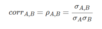
Where ρ(A , B) denotes the covariance among the A and B stocks.
In case,e of low or negative correlations they lower the overall portfolio risk while having no impact on the expected return of our portfolio, as can be shown from our calculation for portfolio risk above. Let’s return to our example for a better understanding.
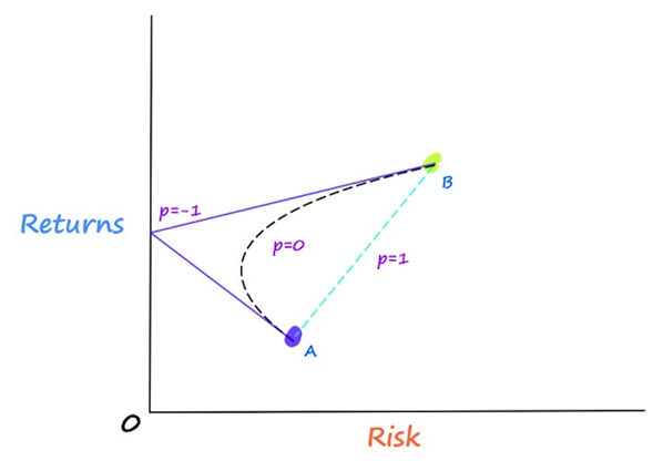
Three distinct situations are shown in the figure above. The highest decrease in the portfolio’s risk occurs when there is a -1 correlation between the two stocks. The risk of our portfolio also rises as a result of the rising stock correlation.
Although this was meant to be a brief introduction to modern portfolio theory, we hope it has given you a basic grasp of the subject so you can learn more about it. The remainder of this blog article will focus on using the PortfolioLab library to implement this portfolio optimization strategy into practice.
Mean-Variance Optimization with PortfolioLab
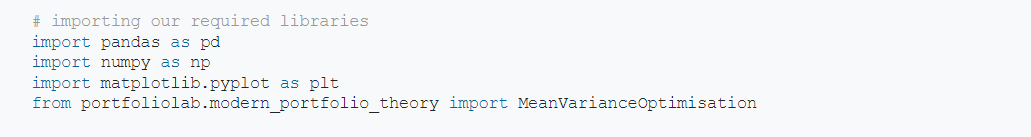
In this part, we’ll demonstrate how customers can employ a variety of mean-variance optimization (MVO) techniques offered by the PortfolioLab Python library to improve their portfolios. Download the required library to carry out tthe optimization process, such as pyPortfolioOpt library or PortfolioLab. We will be using PortfolioLab for this purpose.
Strategies based on Harry Markowtiz’s methodologies for computing effective frontier solutions are used in PortfolioLab’s mean-variance optimization class. Users can create the best portfolio solutions for a variety of objective functions using the PortfolioLab library, such as:
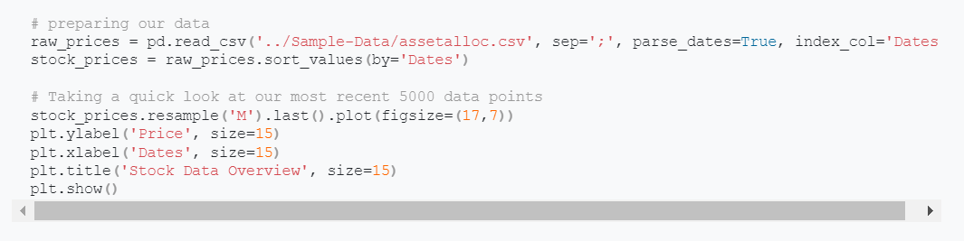
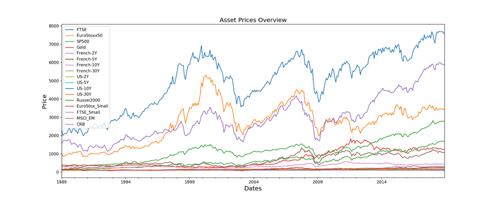
The Data
We’ll be using the previous closing prices for 17 assets in this lesson. The portfolio is made up of a varied range of assets, from bonds to commodities, and each asset has a unique risk-return profile.
Producing a few Sample Portfolios
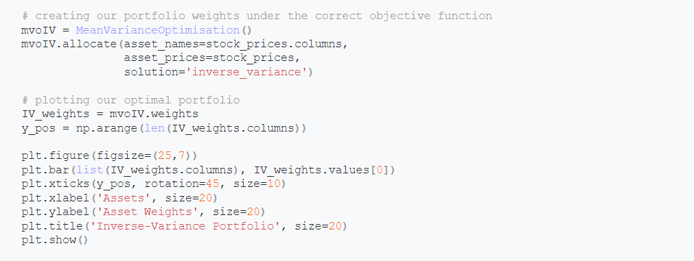
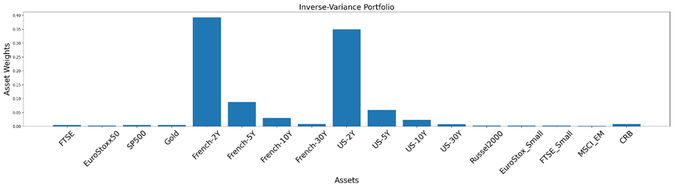
First, we will practice creating an optimal portfolio for the inverse-variance solution string. It’s one of the most straightforward yet effective allocation strategies, outperforming several challenging optimization goals.
We need to make a new MeanVarianceOptimisation object and employ the allocate method to determine the asset weights of the inverse-variance portfolio.
Keep in mind that the allocate method needs the following three parameters to function:
- asset_names (a collection of strings containing the names of the assets).
- asset_prices (a data frame containing historical asset prices – daily close)
- Solution (the kind of solution or algorithm to employ in the weight calculation)
Users can also give expected asset returns and a covariance matrix of asset returns in place of historical asset prices. The allocation mechanism also allows for much more customization. We’ll make it simple for consumers by demonstrating how to build an optimal portfolio using the Inverse Variance portfolio solution. The only thing that needs to be modified to produce a different optimized portfolio is the value of the “solution” parameter string.
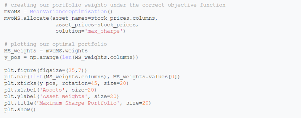
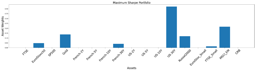
Let’s construct one more portfolio — the highest Sharpe Ratio portfolio. The tangency portfolio may also be used to refer to this.
Custom Input for Users
While many of the calculations needed to construct optimal portfolios are provided by PortfolioLab, users also have the option to give input for their calculations. They can input a covariance matrix of asset returns and the predicted asset returns in place of supplying the raw historical closing prices for their assets to create their optimal portfolio. You can consult the official documentation if you want additional information regarding the customizability within PortfolioLab’s MVO implementation.
The allocate method uses the subsequent parameters to accomplish this:
- ‘covariance_matrix’: (pd.DataFrame/NumPy matrix) a covariance matrix of returns of an asset.
- ‘expected_asset_returns: (list) a lof average asset returns
We will use the ReturnsEstimators class offered by PortfolioLab to perform some of the essential calculations.
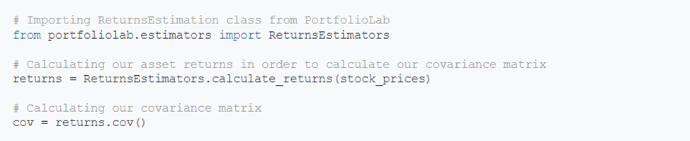
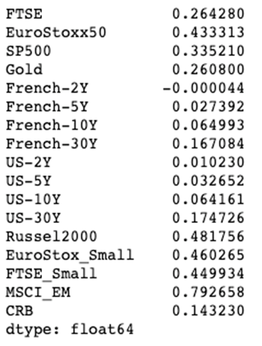
We also determine the anticipated returns or mean asset returns.

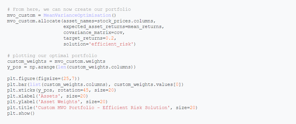
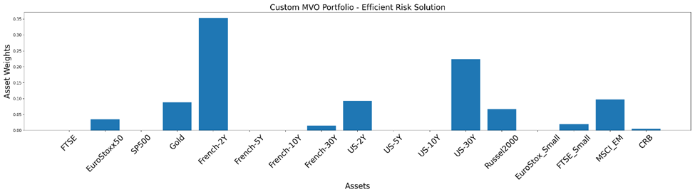
We compute all the necessary input matrices and use these custom inputs to build an effective risk portfolio. The fundamental goal ofan efficient risk portfolio is effective risk management for the investor’s specified target return. In this case, the target return is set to 0.2.
Additionally, many traders and portfolio managers choose to give particular assets in their portfolio a defined weight limit. For example, one would desire to restrict the weights given to French-2Y and US-30Y in the portfolio mentioned above. Let’s attempt to reduce their allocations and slightly diversify the total portfolio. We set a minimum bound on French-5Y and French-10Y and a maximum bound on their weights. Keep in mind that the indexing begins at 0.
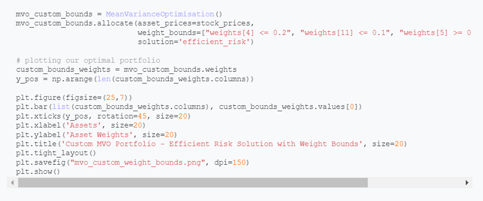
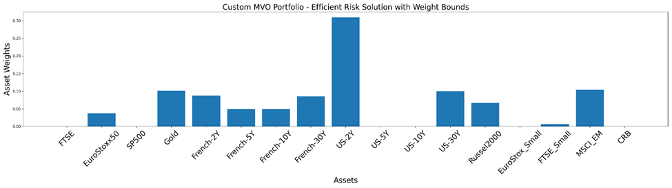
You can observe how the weight bounds assist us in creating a more diverse portfolio and prevent the weights from getting overly centered on a few assets.
The Capital Market Line
The tangent of the efficient frontier is the capital market line. The capital market line (CML) takes its shape from the Capital Asset Pricing Model, which is based on the Modern Portfolio Theory.
The capital market line represents the portfolio’s projected return as a linear of the risk-free rate, the market portfolio’s standard deviation and return, and the portfolio’s standard deviation.
On the efficient frontier, the market portfolio is situated where the line from the risk-free asset (where risk is zero) is tangent to the efficient frontier. Since all assets beneath the efficient frontier offer the same level of return with a greater degree of risk or a lower rate of return with the same level of risk, they are all inefficient portfolios. Conversely, the places above the CML are not reachable.
At the point when the capital market line meets the efficient frontier, all rational investors will hold the combination of risk-free assets and M and the portfolio of risky assets.
Since each investor’s portfolio of risky assets will always be the market portfolio, we can calculate the optimal mix of investments for a portfolio of investors without knowing their levels of risk aversion.
A two-asset portfolio made up of a risk-free asset and a risky asset can be used to calculate the risk-return characteristics provided by CML.
Let’s investigate the following CML equation:
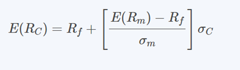
Where:
- E(Rc) is the anticipated return on any portfolio
- Rf is the risk-free return rate
- E(Rm) is the anticipated return on the market portfolio
- σc is the standard deviation of the portfolio’s return
- σm is the standard deviation of the return
The equation may be written as:
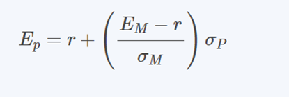
On the capital market line, the factor (Em – r / σM) is equal to the line’s gradient and is commonly referred to as the market price of risk.
As a result, we can write the CML equation above as follows:
Expected return = Market price risk + risk-free rate x Portfolio risk
Investment Strategies
While developing an investment strategy every investor wants to build a portfolio of stocks with the best long-term returns without taking on a lot of risk. The premise of MPT, which incorporates mean-variance analysis, is that investors are risk averse. As a result, they concentrate on developing a portfolio that maximizes the projected returnabouto a particular degree of risk. Investors are aware that high-return investments always carry some risk. Diversifying the portfolio of investments is the answer to reducing risk.
Mutual funds, stocks, bonds, etc., can be included in a portfolio, and each of these financial instruments carries a different level of risk when combined. In an ideal world, a gain in another security would offset a loss in one security’s value.
Comparing a portfolio consisting of more than one type of security to one consisting of only one type is thought to be a better strategic choice. Mean-variance analysis can be a key component of an investment strategy.
Limitations of the Mean-Variance Framework in Portfolio Optimization
Despite being popular, this portfolio optimization strategy has certain drawbacks:
- It is sensitive to input expectations of expected variances, covariances, and expected returns, which are susceptible to uncertainty and minute changes.
- Inadequate portfolio allocations may result from inaccurate estimates. Furthermore, non-normal behavior, skewness, and kurtosis are ignored in the mean-variance optimizer, which assumes that asset returns follow a normal distribution. This may lead toan insufficient assessment of tail risk. optimization assumption made by the optimized strategy is that asset returns would be linear, which may not accurately reflect the complexity of non-linear connections, particularly in the case of options or derivative instruments.
- Additionally, as mean-variance optimization primarily depends on historical data, it may not reliably predict future market circumstances, particularly in the case of structural changes or extreme occurrences.
Conclusion
With the help of mean-variance optimization by PortfolioLab, users can build several common portfolios right away. However, there is also plenty of freedom for those who want to design their portfolio optimization problems with unique constraints, data, and objectives.
Besides, it is imperative to exercise utmost caution. This post is not intended to provide investment advice; rather, it provides a framework for creating your own optimized portfolio with standard examples. To avoid any errors, make sure to update every relevant detail while making any changes to the portfolio optimization.