The success of High-Frequency Trading (HFT) strategies hinges not just on identifying fleeting alpha opportunities, but critically, on the precise and cost-effective execution of orders. While limit orders are the bread and butter of liquidity provision, aggressive market orders are necessary for immediate entry or exit, yet they carry the inherent risk of significant slippage, particularly when dealing with large volumes. Therefore, mastering the art of execution requires rigorous simulation. This article serves as a deep dive into Simulating HFT: A Python Tutorial for Market Order Analysis, providing the quantitative framework necessary to evaluate the true cost of aggressive order flow within complex market microstructures. This specialized analysis extends the core concepts introduced in The Ultimate Guide to Reading the Order Book: Understanding Bid-Ask Spread, Market Liquidity, and Execution Strategy by focusing intensely on the execution mechanics.
Why Simulate HFT Market Order Dynamics?
HFT strategies operate on razor-thin margins. A poorly placed market order, executed during a transient liquidity drought, can instantly wipe out the profit accumulated from numerous successful trades. Simulation allows quants to model execution costs (slippage) under thousands of different order book states (LOBs) and measure the impact of external factors, such as latency and market impact.
The primary goals of Simulating HFT Market Order Analysis are:
- Slippage Quantification: Calculating the realized cost versus the theoretical best price (BBO) when consuming liquidity.
- Liquidity Risk Assessment: Testing how a strategy performs during periods of low liquidity or sudden order book imbalances. This is closely related to the concepts discussed in Order Book Imbalances: A Practical Guide for Day Traders.
- Latency Impact Modeling: Understanding how even minor delays affect the effective price due to rapidly changing LOB conditions.
Prerequisites: Data and Tools for Simulation
Accurate HFT simulation demands high-fidelity data. Standard open/high/low/close data is insufficient. You need time-series data detailing the Limit Order Book (LOB) changes.
Required Data Inputs:
- Full Depth LOB Snapshots (Level 3 Data): While Level 2 data (top 10 bids/asks) is often adequate for general trading, HFT simulation focusing on execution analysis requires deeper insight, ideally mapping the full volume stack to accurately simulate consumption of large market orders.
- Trade Data: Required for validating the simulated LOB evolution between snapshots.
- Timestamp Precision: Nanosecond or microsecond timestamping is non-negotiable, as HFT events unfold within these minuscule timeframes.
Python Environment Setup:
We rely heavily on Python’s scientific stack:
- Pandas: For managing and manipulating large datasets of LOB snapshots.
- NumPy: For vectorizing complex calculations required during market order consumption.
- Custom LOB Class: Creating an object-oriented representation of the order book allows for quick insertion, deletion, and simulation of trades.
Step 1: Modeling the Limit Order Book (LOB) State
The foundation of the simulation is the LOB model. A market order is effectively a demand to be filled immediately at the best available prices on the opposite side of the book until the order size is exhausted.
In Python, we can represent the relevant side of the LOB (e.g., the Ask side for a Buy Market Order) as a structured array or DataFrame, sorted by price:
# Simplified LOB Structure (Ask Side for a Buy Order)
LOB_Ask = [
    {'Price': 100.01, 'Volume': 50},
    {'Price': 100.02, 'Volume': 120},
    {'Price': 100.03, 'Volume': 80},
    # ... deeper levels
]
The Execution Algorithm (Simulating Liquidity Consumption)
When a market order of size Q arrives, the simulation must iterate through the LOB levels, subtracting volume and calculating the Weighted Average Execution Price (WAEP).
The Python function must loop through the price levels until the volume Q is reduced to zero. For each level consumed, the total volume executed and the total cost are tracked. The difference between the Best Ask (BBO) and the WAEP defines the slippage.
For example, if the BBO is $100.01, but a 200-unit market order is filled across $100.01, $100.02, and $100.03, the WAEP will be higher than $100.01, representing the execution cost.
Step 2: Introducing Latency and Execution Risk (The HFT Edge)
For HFT simulations, simply using a static LOB snapshot is insufficient. Latency is the critical variable that determines if the LOB snapshot used for the decision to trade is still valid upon arrival at the exchange.
Assume an HFT firm has 200 microseconds (μs) of total execution latency (time from signal generation to order arrival at the matching engine). During those 200μs, the LOB may have changed dramatically, resulting in “adverse selection” or unexpected high slippage.
Modeling Latency in Python
We simulate latency by looking forward in our data stream. If a trade decision is made at time $T$, we check the actual LOB state at time $T + \Delta t_{latency}$.
A fundamental function in the simulation should be:
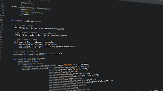
def get_realized_lob(initial_timestamp, latency_ms, LOB_data_stream):
    """Retrieves the LOB state as it would appear upon order arrival."""
    arrival_time = initial_timestamp + timedelta(microseconds=latency_ms)

    # Find the closest LOB snapshot *after* the arrival time
    realized_lob = LOB_data_stream.loc[LOB_data_stream.index >= arrival_time].iloc[0]

    return realized_lob
By comparing the slippage calculated on the pre-execution LOB (what the algorithm saw) versus the slippage calculated on the realized LOB (what the exchange saw), we quantify the impact of latency. This level of precision is necessary when studying the complex interactions described in The Game Theory of HFT: How Exchanges, Algorithms, and Investors Interact.
Python Tutorial: Analyzing Market Order Impact
Our focus here is generating a metric called the Market Order Impact Index (MOII), which measures the price perturbation caused by a fixed market order size (e.g., 1000 shares) across various market conditions.
Step 3: Calculating Slippage and Market Impact
We define slippage (S) as the difference between the Best Available Price (BAP) at the time of signal generation and the Weighted Average Execution Price (WAEP).
$$ S = WAEP – BAP $$
The WAEP is calculated as:
$$ WAEP = \frac{\sum (Price_i \times Volume_i)}{\sum Volume_i} $$
Example Python Implementation (Conceptual):
def calculate_waep_and_slippage(order_size, current_lob_side, initial_bbo):

    remaining_size = order_size
    total_cost = 0
    total_filled = 0

    for level in current_lob_side:
        price = level['Price']
        available_volume = level['Volume']

        fill_volume = min(remaining_size, available_volume)

        total_cost += price * fill_volume
        total_filled += fill_volume
        remaining_size -= fill_volume

        if remaining_size <= 0:
            break

    if total_filled > 0:
        waep = total_cost / total_filled
        slippage = waep - initial_bbo
        return waep, slippage
    else:
        return initial_bbo, 0.0 # Should not happen unless book is empty
By running this function iteratively over thousands of LOB snapshots, we build a statistical distribution of potential execution costs for a given order size, which is crucial for determining optimal execution strategies, particularly in volatile markets like those seen in Order-Book Perpetuals: A New Playbook for Crypto Traders.
Case Study: Measuring Slippage Across Different Liquidity States
To showcase the utility of the simulation, consider a scenario where a high-frequency strategy needs to execute a standard 500-unit market order.
Scenario A: Deep, Tight Market (High Liquidity)
LOB State (Ask Side): BBO = 10.00. Deep volume clustered tightly around 10.00 and 10.01.
- 500 units filled at WAEP = 10.002.
- Slippage: 0.002 (2 basis points). Minimal impact.
Scenario B: Shallow, Wide Market (Low Liquidity)
LOB State (Ask Side): BBO = 10.00. Immediate volume scarcity, large jumps in price.
| Price | Volume | Cumulative Volume |
|---|---|---|
| 10.00 | 50 | 50 |
| 10.01 | 50 | 100 |
| 10.05 | 100 | 200 |
| 10.10 | 300 | 500 (Filled) |
In Scenario B, the order consumed liquidity spanning 10 ticks (10.00 to 10.10). The resulting WAEP would be significantly higher (around 10.076).
- 500 units filled at WAEP ≈ 10.076.
- Slippage: 0.076 (7.6 basis points). High impact.
Actionable Insight: By simulating these scenarios, the HFT algorithm can learn to dynamically adjust its order size or choose a passive execution strategy (aggressive limit order) when the calculated slippage exceeds a predetermined maximum threshold. This highlights why understanding the depth of the LOB, not just the BBO, is essential—a concept often overlooked in simple BBO-based strategies. Analyzing such execution risks is particularly relevant when dealing with varying market structures, such as those analyzed in How the Bid-Ask Spread Actually Works in Crypto vs. Stocks.
Conclusion
Simulating HFT: A Python Tutorial for Market Order Analysis provides the necessary quantitative tools to transform raw order book data into actionable intelligence regarding execution efficiency. By accurately modeling the LOB state, introducing realistic latency, and calculating the Weighted Average Execution Price (WAEP), quantitative traders can rigorously test the robustness of their strategies against the unavoidable costs of liquidity consumption. Minimizing slippage through sophisticated simulation is often the difference between a profitable HFT operation and one that consistently underperforms.
For a broader understanding of how these execution mechanics fit into the overall market landscape, revisit the foundational principles covered in The Ultimate Guide to Reading the Order Book: Understanding Bid-Ask Spread, Market Liquidity, and Execution Strategy.
Frequently Asked Questions (FAQ)
What is the primary difference between simulating limit orders and simulating market orders?
Simulating limit orders focuses on queue position and fill probability—modeling how long the order waits and if it gets hit before the price moves away. Simulating market orders focuses exclusively on immediate execution cost, measuring the depth of the book consumed and the resulting slippage incurred by consuming that volume.
Why is nanosecond timestamp resolution crucial for HFT market order simulation?
In HFT, market conditions can change completely within milliseconds due to other high-speed participants updating the LOB. Nanosecond resolution ensures that the simulator accurately captures the LOB state at the exact moment the order is presumed to hit the exchange, allowing for precise latency modeling and slippage calculation.
How does LOB depth data (Level 3) improve market order analysis compared to Level 2 data?
Level 2 data provides only a limited view (e.g., 10 price levels). If a large market order exceeds the volume available in those 10 levels, Level 2 data cannot accurately calculate the resulting slippage. Level 3 data, which maps all visible volume, is required to simulate the full consumption path and calculate the true Weighted Average Execution Price (WAEP).
What is the Market Order Impact Index (MOII) and how is it used in simulations?
The MOII is a synthetic metric derived from simulation that quantifies the price movement caused by a standard unit of market order flow (e.g., a 1,000-share market order). It is used to gauge market fragility and liquidity risk, helping algorithms adjust order sizing dynamically. A high MOII suggests low liquidity and high potential slippage.
Can this simulation methodology be applied to complex instruments like options or perpetuals?
Yes. While the structure of the order book for instruments like options can be more complex (see: Trading Complex Order Books in Options), the core methodology remains the same: map the volume stack, simulate sequential consumption based on the order size, and calculate the WAEP. This is vital for complex derivatives where liquidity can be highly fragmented.
How does adverse selection relate to market order simulation latency?
Adverse selection occurs when a trade is executed based on stale information. In simulation, if a delay (latency) exists, the LOB seen by the algorithm might show high liquidity, but the LOB upon arrival (the realized LOB) might be empty or thin, leading to unexpectedly high slippage. Simulation quantifies the likelihood and severity of this adverse selection based on historical market volatility and observed latency.


